
In my last post I introduced the concept of using network analysis for use on Road data. In another post I looked at using pygeos to spatially smooth data. This time I’ll be combining network analysis and spatial smoothing.
The Problem
Using distance related spatial smoothing, whether this is using kernel density or count/average within a radius, can have potential issues. It also has advantages over what I’m about to cover but I’m going to ignore them. Let’s say I’m looking at the average house price in an area. If I was in Central London I might call within 500m my local neighbourhood. But in a village 500m isn’t very far and you might extend it to include some of the other local villages, so a fixed distance very good.
My Solution
You could just use postcode, start at within your postcode, then sector, district and area. But if you live on the boundary between two districts or areas it means a reasonable chunk of your neighbourhood will be ignored.
My idea is to use the census LSOA areas. Each of these should contain roughly the same number of people/houses. The mean population (in 2011) in each one is about 1500. I want to take a map of these and then aggregate up to bigger neighbourhoods based on the boundaries of that LSOA. Then we can make neighbourhoods within 1, 2, 3, …etc. LSOAs of the original one.
Method
First, get a map of the LSOAs. Luckily I have these already from this post on mapping UK open data in python. Below is a map of the LSOAs around St Paul’s Cathedral.

Generate spatial weights diagram using Queen neighbours (neighbours only need to share a vertex, it would be a rook neighbour if they had to share an edge). This is done using the libpysal package. We then convert the diagram into a networkx network diagram and store the centroid positions for plotting later.
centroids = np.column_stack((LSOA.centroid.x, LSOA.centroid.y))
queen = weights.Queen.from_dataframe(LSOA)
G = queen.to_networkx()
positions = dict(zip(G.nodes, centroids))

Which gives this rather nice set of pictures. There is already an issue with this that is immediately apparent. It doesn’t work for non-contiguous boundaries. I don’t know how to fix that. I somehow need to add in bridges. Now I’ve raised that issue, lets forget about it and pretend it’s not an issue.
Side note
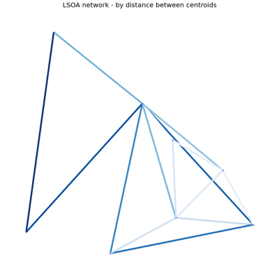
As with the diagrams used for roads you can apply attributes to the edges and nodes and use that for plotting. In this case storing the distance between centroids on the edges and colouring the edges accordingly

The next picture shows the same code run over the same area of land, but this time centred on Windermere.
As you can see. The number rural nature of the area translates into a much simpler graph.
Back to the original chain of thought
Now that we have our network diagram we can use the ego_graph function to find the nodes within 1, 2 and 3 edges of a given node. Or, for our LSOAs: we can find the LSOAs within 1, 2 or 3 boundaries of our original LSOA

Finally, we can put all of these on a single plot

You can then use these subnetworks to spatially smooth the data for within each LSOA.
As with my previous post you can find the notebook with all of the code for this post here.